
Reserves estimates drive company valuations, lending, acquisitions and national planning, so the way they are classified matters as much as the way they are calculated. In January 2004 Shell announced that about 20% of its end-2002 proved reserves (some 3.9 billion barrels of oil equivalent) did not meet the SEC definition of proved; later revisions brought the cut to about 29%, and the company paid $120 million to the SEC and £17 million to the UK Financial Services Authority to settle the resulting cases. This guide explains the SPE Petroleum Resources Management System (PRMS), the volumetric and material balance methods, and the reporting rules that sit on top of them, with one synthetic example throughout.
1. The PRMS classification
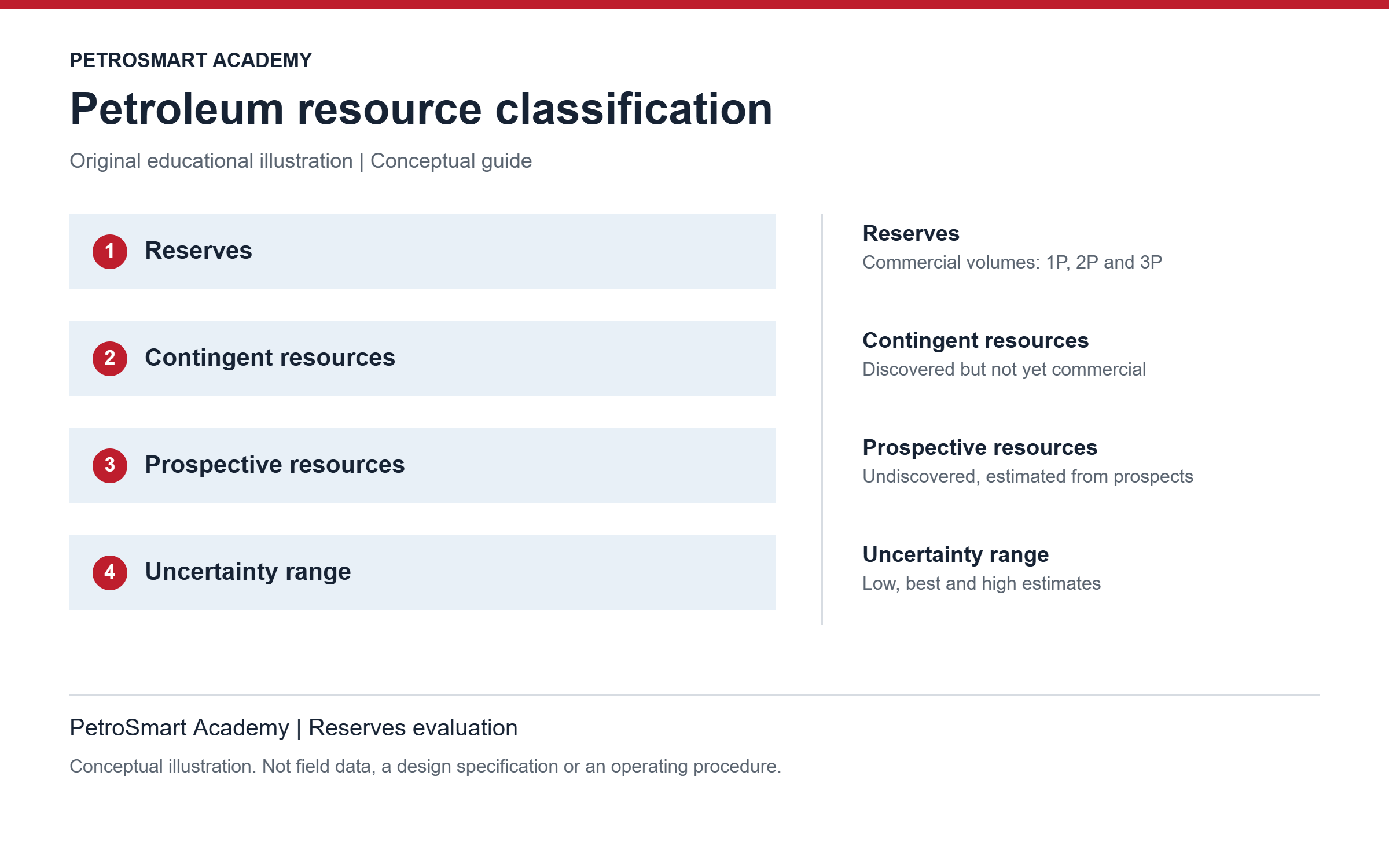
PRMS (SPE, 2018 update) classifies recoverable quantities along two axes: the chance that a project will be commercial, and the uncertainty in the quantity recovered.
| Class | Meaning | Uncertainty categories |
|---|---|---|
| Reserves | Discovered, commercially recoverable quantities from a project justified for development, with a reasonable expectation that it will proceed | Proved (1P), Proved + Probable (2P), Proved + Probable + Possible (3P) |
| Contingent resources | Discovered quantities whose development is not yet commercial because of one or more contingencies (technical, commercial, regulatory) | 1C, 2C, 3C |
| Prospective resources | Undiscovered quantities estimated for prospects; they carry a chance of discovery and a chance of development | 1U, 2U, 3U (low, best, high) |
When probabilistic methods are used, there should be at least a 90% probability that the quantity actually recovered will equal or exceed the 1P estimate (P90), at least 50% for 2P (P50) and at least 10% for 3P (P10). Probable and Possible reserves are the increments 2P − 1P and 3P − 2P; the probability statements apply to the cumulative totals, not to the increments themselves. P90 is therefore always the low estimate and P10 the high estimate. Proved reserves are further split into developed producing, developed non-producing and undeveloped.
2. Volumetric estimate of oil in place
STOIIP (STB) = 7,758 × A × hnet × φ × (1 − Swi) / Boi
with A in acres, hnet in feet, 7,758 bbl per acre-foot. For gas, GIIP (scf) = 43,560 × A × hnet × φ × (1 − Swi) / Bgi, with Bgi = 0.02827 z T / p in ft³/scf (T in °R, p in psia).
Synthetic example. A = 8,450 acres, gross thickness 285 ft with net-to-gross 0.68 (hnet = 193.8 ft), φ = 0.192, Swi = 0.285, Boi = 1.365 RB/STB. Deterministic STOIIP = 7,758 × 8,450 × 193.8 × 0.192 × 0.715 / 1.365 = 1,278 MMstb.
Monte Carlo. With triangular distributions (low, most likely, high) of A = 7,200 / 8,450 / 9,800 acres, hnet = 155 / 194 / 235 ft, φ = 0.168 / 0.192 / 0.218, Swi = 0.250 / 0.285 / 0.325 and Boi = 1.340 / 1.365 / 1.392, 200,000 trials give STOIIP P90 = 1,094, P50 = 1,283 and P10 = 1,494 MMstb (mean 1,290). Because inputs are combined at random, the P90 of the result is much less extreme than a case built with every input at its low value.
3. From oil in place to reserves
Recovery factor is the product of displacement efficiency (the fraction of oil displaced from the pores that the injected water actually contacts) and volumetric sweep efficiency (the fraction of the reservoir volume contacted). With Swi = 0.285 and a residual oil saturation of 0.25 to water, the maximum displacement efficiency is ED = (1 − 0.285 − 0.25) / (1 − 0.285) = 65%. That is not a field recovery factor: with a volumetric sweep of 0.65 the waterflood recovery would be about 42% before economic limits.
Reserves are computed by combining distributions, not by multiplying percentiles. Treating recovery factor as triangular (0.35 / 0.42 / 0.50) and combining it with the STOIIP distribution gives, for a project that qualifies as Reserves, 1P ≈ 451, 2P ≈ 541 and 3P ≈ 647 MMstb. Multiplying the P90 STOIIP by the low recovery factor would give 383 MMstb, an estimate far below the true P90.
4. Aggregating fields
Field X has 1P / 2P / 3P of 50 / 75 / 120 MMstb and field Y 30 / 45 / 70 MMstb. Fitting a lognormal distribution to each field's P90 and P10 and adding the two independent distributions by Monte Carlo gives a portfolio P90 of about 92, P50 of 126 and P10 of 175 MMstb, against arithmetic sums of 80 and 190. The probabilistic P90 of a sum is higher than the sum of the P90s, and the P10 lower, because both fields are unlikely to disappoint (or surprise) together. This only holds if the fields are truly independent; shared uncertainties such as price, a common fluid model or the same interpretation method create correlation.
Arithmetic summation is not "wrong": it is the conservative method that PRMS recognizes and that reporting rules usually require for disclosure, while statistical aggregation is useful for internal portfolio analysis. Whichever is used must be stated.
5. Checking in-place volumes with material balance
Once pressure and production data exist, the Havlena-Odeh form of the material balance tests the volumetric estimate. For an oil reservoir without gas cap or aquifer, and neglecting rock and water compressibility below the bubble point:
F = N Eo, with F = Np[Bo + (Rp − Rs)Bg] + WpBw and Eo = (Bo − Boi) + (Rsi − Rs)Bg
Synthetic data after Np = 45.2 MMstb, pressure down from 4,620 to 3,850 psia: Bo = 1.318, Boi = 1.365 RB/STB, Rs = 485, Rsi = 580, Rp = 625 scf/STB, Bg = 0.00142 RB/scf, no water produced. Then Eo = −0.047 + 95 × 0.00142 = 0.0879 RB/STB, F = 45.2 × 10⁶ × 1.5168 = 68.6 × 10⁶ RB, and N = F / Eo ≈ 780 MMstb.
One point proves little; the method needs several surveys plotted as F against Eo. A straight line through the origin supports the no-aquifer model; upward curvature points to water influx, which would make 780 MMstb an overestimate of the connected oil. Here the result is far below the volumetric P90 of 1,094 MMstb, so the subsurface model must be reviewed (compartments, net pay, porosity, pressure data quality) before more reserves are booked.
6. Reporting rules: the SEC example
Companies listed in the United States report under SEC Regulation S-X Rule 4-10(a), modernized in 2008:
- Reasonable certainty: when probabilistic methods are used, at least a 90% probability that quantities recovered will equal or exceed the estimate.
- Fluid contacts: without data on a contact, proved quantities are limited to the lowest known hydrocarbons, unless geoscience, engineering or performance data and reliable technology establish a lower contact with reasonable certainty.
- Undeveloped reserves: proved undeveloped locations must be scheduled for drilling within five years, unless specific circumstances justify a longer time.
- Prices: economic producibility is tested with the unweighted average of first-day-of-the-month prices over the preceding twelve months.
Requirements for independent evaluation differ by jurisdiction. The SEC does not require a third-party audit, but a company that states it used one must disclose the evaluator's report. Canada's National Instrument 51-101, by contrast, requires reporting issuers to have reserves evaluated or audited by independent qualified reserves evaluators. SPE publishes standards for estimating and auditing reserves information.
7. Portfolio metrics
- Reserves life index = proved reserves / annual production. Example: 2,850 / 180 MMstb per year = 15.8 years.
- Reserves replacement ratio = reserves added / production. Example: 215 / 180 = 1.19. Over several years, divide total additions by total production rather than averaging yearly ratios (with equal yearly production of 180 MMstb and ratios of 0.85, 1.42 and 1.19, the result is 1.15 either way, but not when production varies).
- Finding and development cost = exploration and development spending / reserves added. Example: $850M / 320 MMstb = $2.66/bbl. Compare it only with companies using the same definitions and time period.
References
- SPE/WPC/AAPG/SPEE/SEG/SPWLA/EAGE, Petroleum Resources Management System (2018)
- US SEC, Modernization of Oil and Gas Reporting (2008) and Regulation S-X Rule 4-10
- Canadian Securities Administrators, NI 51-101
- D. Havlena and A.S. Odeh, "The Material Balance as an Equation of a Straight Line", JPT (1963). Shell figures: Oil & Gas Journal reporting of the SEC and FSA settlements (2004)
Related reading and community
Questions or field experience to share? Join the PetroSmart Telegram group, watch worked examples on the PetroSmart Academy YouTube channel and follow us on Facebook.